Introdução

Como foi dito na página de métodos estatísticos, a análise estatística multivariada utilizando funções discriminantes foi inicialmente aplicada para decidir à qual de dois grupos pertenceriam indivíduos sobre os quais tinham sido feitas diversas e idênticas mensurações.

Nessa análise, hoje conhecida como análise discriminante linear, a idéia básica é substituir o conjunto original das diversas mensurações por um único valor D_i, definido como uma combinação linear delas. Quando se trata de discriminar entre mais de dois grupos torna-se necessário uma generalização na metodologia. A análise discriminante multigrupos, que utiliza procedimentos combinados da análise de variância e da análise fatorial, pode, então, ser utilizada. 

Nesta página vamos ver como se uytiliza a Análise de Discriminantes através de exemplos.

Primeiro Exemplo Detalhado: Discriminação entre portadores ou não de Hemofilia

Tomemos para isso o seguinte exemplo:

Grupo 1: mulheres não portadoras de hemofilia A (normais) (n1 = 30)
Grupo 2: mulheres portadoras de hemofilia A (portadoras)  (n2 = 22)
Suponha que as variáveis discriminadoras são: X1 e X2 (duas variáveis contínuas observadas em exames de sangue). No nosso exemplo vamos considerar somente essas.

Os dados são:

dados

Um scatter plot da distribuição dos dados fica assim:

Scatter plot

Scatter plot

Formas de Análise de Discriminantes

Estime os coeficientes da função discriminante e determine a significância estatística e a validade — escolha o método de análise de discriminantes apropriado.

• The direct method involves estimating the discriminant function so that all the predictors are assessed simultaneously. The stepwise method enters the predictors sequentially.
• The two-group method should be used when the dependent variable has two categories or states.
• The multiple discriminant method is used when the dependent variable has three or more categorical states.

Análise de Discriminates sobre uma única Variável

the final significance test of whether or not a variable discriminates between groups is the F test.  F is essentially computed as the ratio of the between-groups variance in the data over the pooled (average) within-group variance.  If the between-group variance is significantly larger then there must be significant differences between means.

Análise de Discriminantes com Múltiplas Variáveis

Usually, one includes several variables in a study in order to see which one(s) contribute to the discrimination between groups.  In that case, we have a matrix of total variances and covariances; likewise, we have a matrix of pooled within-group variances and covariances.  We can compare those two matrices via multivariate F tests in order to determined whether or not there are any significant differences (with regard to all variables) between groups.  This procedure is identical to multivariate analysis of variance or MANOVA.  As in MANOVA, one could first perform the multivariate test, and, if statistically significant, proceed to see which of the variables have significantly different means across the groups.  Thus, even though the computations with multiple variables are more complex, the principal reasoning still applies, namely, that we are looking for variables that discriminate between groups, as evident in observed mean differences.  In fact, you may perform discriminant function analysis with the ANOVA/MANOVA module; however, different types of statistics are customarily computed and interpreted in discriminant analysis (as described later).

Pressupostos Fundamentais por Detrás da Análise de Discriminantes

Discriminant function analysis is computationally very similar to MANOVA, and all assumptions for MANOVA mentioned in ANOVA/MANOVA apply. In fact, you can use the wide range of diagnostics and statistical tests of assumption that are available in ANOVA/MANOVA to examine your data for the discriminant analysis (to avoid unnecessary duplications, the extensive set of facilities provided in ANOVA/MANOVA is not repeated in Discriminant Analysis):

• Normal distribution. It is assumed that the data (for the variables) represent a sample from a multivariate normal distribution. Note that it is very simple to produce histograms of frequency distributions from within results spreadsheets via the shortcut menu, which allows you to examine whether or not variables are normally distributed. However, note that violations of the normality assumption are usually not “fatal,” meaning, that the resultant significance tests etc. are still “trustworthy.” ANOVA/MANOVA provides specific tests for normality.
• Homogeneity of variances/covariances. It is assumed that the variance/covariance matrices of variables are homogeneous across groups. Again, minor deviations are not that important; however, before accepting final conclusions for an important study it is probably a good idea to review the within-groups variances and correlation matrices. In particular the scatterplot matrix that can be produced from the Prob. and Scatterplots tab of the Descriptive Statistics dialog can be very useful for this purpose. When in doubt, try re-running the analyses excluding one or two groups that are of less interest. If the overall results (interpretations) hold up, you probably do not have a problem. You may also use the numerous tests and facilities in ANOVA/MANOVA to examine whether or not this assumption is violated in your data. However, as mentioned in ANOVA/MANOVA, the multivariate Box M test for homogeneity of variances/covariances is particularly sensitive to deviations from multivariate normality, and should not be taken too “seriously.”
• Correlations between means and variances. The major “real” threat to the validity of significance tests occurs when the means for variables across groups are correlated with the variances (or standard deviations). Intuitively, if there is large variability in a group with particularly high means on some variables, then those high means are not reliable. However, the overall significance tests are based on pooled variances, that is, the average variance across all groups. Thus, the significance tests of the relatively larger means (with the large variances) would be based on the relatively smaller pooled variances, resulting erroneously in statistical significance. In practice, this pattern may occur if one group in the study contains a few extreme outliers, who have a large impact on the means, and also increase the variability. To guard against this problem, inspect the descriptive statistics, that is, the means and standard deviations or variances for such a correlation. ANOVA/MANOVA also allows you to plot the means and variances (or standard deviations) in a scatterplot.
• The matrix ill-conditioning problem. Another assumption of discriminant function analysis is that the variables that are used to discriminate between groups are not completely redundant. As part of the computations involved in discriminant analysis, STATISTICA inverts the variance/covariance matrix of the variables in the model. If any one of the variables is completely redundant with the other variables then the matrix is said to be ill-conditioned, and it cannot be inverted. For example, if a variable is the sum of three other variables that are also in the model, then the matrix is ill-conditioned.
• Tolerance values. In order to guard against matrix ill-conditioning, STATISTICA constantly checks the so-called tolerance value for each variable. This value is also routinely displayed when you ask to review the summary statistics for variables that are in the model, and those that are not in the model. This tolerance value is computed as 1 minus R-square of the respective variable with all other variables included in the current model. Thus, it is the proportion of variance that is unique to the respective variable. You can also refer to Multiple Regression to learn more about multiple regression and the interpretation of the tolerance value. In general, when a variable is almost completely redundant (and, therefore, the matrix ill-conditioning problem is likely to occur), the tolerance value for that variable will approach 0. The default value in Discriminant Analysis for the minimum acceptable tolerance is 0.01. STATISTICA issues a matrix ill-conditioning message when the tolerance for any variable falls below that value, that is if any variable is more than 99% redundant (you may change this default value by selecting the Advanced options (stepwise analysis) check box on the Quick tab of the Discriminant Function Analysis dialog, and then adjusting the Tolerance box on the resulting Advanced tab of the Model Definition dialog).

Análise de Discriminantes do Tipo Passo a Passo

Probably the most common application of discriminant function analysis is to include many measures in the study, in order to determine the ones that discriminate between groups. For example, an educational researcher interested in predicting high school graduates’ choices for further education would probably include as many measures of personality, achievement motivation, academic performance, etc. as possible in order to learn which one(s) offer the best prediction.

Model. Put another way, we want to build a “model” of how we can best predict to which group a case belongs. In the following discussion we will use the term “in the model” in order to refer to variables that are included in the prediction of group membership, and we will refer to variables as being “not in the model” if they are not included.

Forward stepwise analysis. In stepwise discriminant function analysis, STATISTICA “builds” a model of discrimination step-by-step. Specifically, at each step STATISTICA reviews all variables and evaluate which one will contribute most to the discrimination between groups. That variable will then be included in the model, and STATISTICA proceeds to the next step.

Backward stepwise analysis. You can also step backwards; in that case STATISTICA first includes all variables in the model and then, at each step, eliminates the variable that contributes least to the prediction of group membership. Thus, as the result of a successful discriminant function analysis, one would only keep the “important” variables in the model, that is, those variables that contribute the most to the discrimination between groups.

F to enter, F to remove. The stepwise procedure is “guided” by the respective F to enter and F to remove values. The F value for a variable indicates its statistical significance in the discrimination between groups, that is, it is a measure of the extent to which a variable makes a unique contribution to the prediction of group membership. If you are familiar with stepwise multiple regression procedures (see Multiple Regression), then you may interpret the F to enter/remove values in the same way as in stepwise regression.

In general, STATISTICA continues to choose variables to be included in the model, as long as the respective F values for those variables are larger than the user-specified F to enter; STATISTICA excludes (removes) variables from the model if their significance is less than the user-specified F to remove.

Capitalizing on chance. A common misinterpretation of the results of stepwise discriminant analysis is to take statistical significance levels at face value. When STATISTICA decides which variable to include or exclude in the next step of the analysis, it actually computes the significance of the contribution of each variable under consideration. Therefore, by nature, the stepwise procedures will capitalize on chance because they “pick and choose” the variables to be included in the model so as to yield maximum discrimination. Thus, when using the stepwise approach you should be aware that the significance levels do not reflect the true alpha error rate, that is, the probability of erroneously rejecting H0 (the null hypothesis that there is no discrimination between groups).

Como Interpretar uma Função Discriminante entre Dois Grupos?

In the two-group case, discriminant function analysis can also be thought of as (and is analogous to) multiple regression (see Multiple Regression; the two-group discriminant analysis is also called Fisher linear discriminant analysis after Fisher, 1936; computationally all of these approaches are analogous). If we code the two groups in the analysis as 1 and 2, and use that variable as the dependent variable in a multiple regression analysis, then we would get results that are analogous to those we would obtain via Discriminant Analysis. In general, in the two-group case we fit a linear equation of the type:

Group = a + b1*x1 + b2*x2 + … + bm*xm

where a is a constant and b1 through bm are regression coefficients. The interpretation of the results of a two-group problem is straightforward and closely follows the logic of multiple regression: Those variables with the largest (standardized) regression coefficients are the ones that contribute most to the prediction of group membership.

Análise de Discrimantes para Determinação de Funções Discriminantes entre Vários Grupos

When there are more than two groups, we can estimate more than one discriminant function like the one presented above. For example, when there are three groups, we could estimate (1) a function for discriminating between group 1 and groups 2 and 3 combined, and (2) another function for discriminating between group 2 and group 3. We could have one function that discriminates between those high school graduates that go to college and those who do not (but rather get a job or go to a professional or trade school), and a second function to discriminate between those graduates that go to a professional or trade school versus those who get a job. The b coefficients in those discriminant functions could then be interpreted as before.

• Análise Canônica: When actually performing a multiple group discriminant analysis, we do not have to specify how to combine groups so as to form different discriminant functions. Rather, STATISTICA automatically determines some optimal combination of variables so that the first function provides the most overall discrimination between groups, the second provides second most, and so on. Moreover, the functions will be independent or orthogonal, that is, their contributions to the discrimination between groups will not overlap. Computationally, STATISTICA performs a canonical correlation analysis (see also Canonical Correlation) that will determine the successive functions and canonical roots (the term root refers to the eigenvalues that are associated with the respective canonical function). The maximum number of functions that STATISTICA computes are equal to the number of groups minus one, or the number of variables in the analysis, whichever is smaller.
• Interpretação das Funções Discriminantes: As before, we get b (and standardized Beta) coefficients for each variable in each discriminant (now also called canonical) function, and they can be interpreted as usual: the larger the standardized coefficient, the greater is the contribution of the respective variable to the discrimination between groups. (Note that we could also interpret the structure coefficients; see below.) However, these coefficients do not tell us between which of the groups the respective functions discriminate. We can identify the nature of the discrimination for each discriminant (canonical) function by looking at the means for the functions across groups. We can also visualize how these two functions discriminate between groups by plotting the individual scores for the two discriminant functions.
• Significância das Funções Discriminantes: One can test the number of roots that add significantly to the discrimination between group. Only those found to be statistically significant should be used for interpretation; non-significant functions (roots) should be ignored.

Resumindo, when interpreting multiple discriminant functions, which arise from analyses with more than two groups and more than one variable, you would first test the different functions for statistical significance, and only consider the significant functions for further examination. Next, you would look at the standardized b coefficients for each variable for each significant function. The larger the standardized b coefficient, the larger is the respective variable’s unique contribution to the discrimination specified by the respective discriminant function. In order to derive substantive “meaningful” labels for the discriminant functions, you can also examine the factor structure matrix with the correlations between the variables and the discriminant functions. Finally, you would look at the means for the significant discriminant functions in order to determine between which groups the respective functions seem to discriminate.

Segundo Exemplo Detalhado: Discriminando Diferentes Variedades da Flor Iris

Para exemplificar a utilização de análise de discriminates vamos nos basear em um conjunto de dados bastante utilizado para demonstrar Análise de Disciminantes: o conjunto de dados sobre três espécies de flores do gênero Iris, Iris setosa (comum nos jardins da nossa ilha), Iris versicolor e Iris virginica. Estes dados foram colhidos por Fisher em 1936 e até hoje servem de exemplo de como se pode escolher funções discriminantes para um conjunto de dados composto por três classes. Os dados descrevem 150 espécimes de Iris de acordo com 4 características: comprimento das sépalas, comprimento das pétalas, largura das sépalas e largura das pétalas. A quinta váriável é a variável de grupo ou variável categórica, que associa a classificação a cada espécime ou caso observado. Apresentamos uma parte desse conjunto de dados abaixo:

Dados Íris

O nosso desafio será encontrar alguma forma de discriminar entre novos espécimes de Iris com base nessa informação acima.

Dados Íris

Dados Íris

Dados Íris

Dados Íris

Exercício de Análise de Discriminantes

Procure nos Links Úteis da página por fontes de software livre para Análise de Discriminantes.  Escolha um software livre de sua preferência, baixe-o e instale-o em seu computador ou no laboratório.

A seguir, tome um conjunto de quatro sets de dados, dentre estes:

• Os dados da flor do Gênero Iris disponíveis nesta página ou em muitos repositórios de dados para teste de software estatístico.
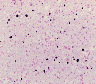
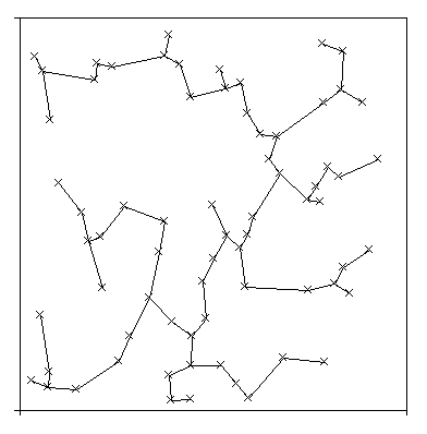
• Os dados dos casos de câncer cerebral (gliomas) que serão fornecidos. Para você entender o câncer da glia e a classificação em graus de malignidade e o método utilizado para a geração dos dados que você vai baixar no link abaixo, veja uma explicação detalhada do trabalho aqui. Resumidamente podemos dizer que no câncer cerebral mais comum, o que ocorre nas células gliais ou de suporte do cérebro, o fator mais importante a ser determinado é a taxa de crescimento do tumor, o que vai determinar a forma de tratamento. Isto é chamado de gradação do tumor. Determinar esta taxa depende de uma série de fatores que um patologista experiente é capaz de identificar em uma lâmina de uma biópsia cerebral. Extraindo-se dados com análise de iamgesn e classificando-se estatisticamente estes dados pode-se chegra a resultados similares. Dados de 680 lâminas histopatológicas de 170 pacientes (4 por paciente) obtidas por estereotaxia coloridas com KI97 e Feulgen. Colunas da esquerda: parâmetros de análise de imagens obtidos automaticamente e teoricamente descritivos. Colunas da direita: Resultados da classificaçao manual em 1993/1995 por Dr. Harry Kolles e Prof. Feiden da Universidade de Homburg, Alemanha de acordo com a nova escala em estudo pela OMS denominada escala Saint-Anne/Mayo ou escala Daumas-Duport. Hoje padrão da OMS

Tumor da Glia (glioma). Lâmina colorida com corante que mostra as células em divisão.	Árvore Expandida de Custo Mínimo (mst) descrevendo a relação espacial entre as células cancerosas.

• Outros dois conjuntos quaisquer que você deverá procurar também nos Links Úteis.

Realize dois conjuntos de Análises de Discriminantes sobre estes sets de dados:

• Um deles buscando uma variável discriminatória para divisão em apenas dois grupos
• Outra multigrupos, buscando o conjunto de funções discriminatórias.
• No último caso utilize apenas metade dos dados para a A.D., utilizando então as funções geradas para classificar os dados restantes. Verifique a acurácia de sua classificação.

Produza um relatório descrevendo: a) os resultados que obteve e as conclusões que tirou disso e b) a sua experiência na utilização do software livre estatístico em questão.