A Segmentação Hierárquica Recursiva (RHSEG) é um algoritmo de processamento de imagens desenvolvido no NASA Goddard Space Flight Center. É uma melhoria do Método de Segmentação Hierárquica com Agrupamento Espectral (HSEG), o qual, por sua vez, é uma melhoria do Método de Segmentação Hierárquica por Otimização Passo-a-Passo (HSWO). Vamos ver cada um deles a seguir.
Contents
Componentes do RHSEG
Método de Segmentação Hierárquica por Otimização Passo-a-Passo (HSWO)
The primary flaw with the previous region growing approaches is that the segmentation produced by these approaches is non-optimal, thus are not unique. The number and shape of the partitions depend on the order in which the image is scanned and processed. The concept of optimality is not present as any partition that satisfies the conditions represent an equally valid segmentation of the image. This is where the Hierarchical Step-Wise Optimization provides a much more optimal solution.
In the first step, the algorithm initializes the segmentation by labeling each pixel. If a pre-segmentation exists, each pixel is labeled according to the pre-segmentation. Otherwise, each pixel is labeled as a separate region. In the second step, it calculates the dissimilarity criterion value between all pairs of spatially adjacent regions, finds the pair of spatially adjacent regions with the smallest dissimilarity value, and merges that pair of regions. In the third step, the algorithm stops if no more merges are required, otherwise it returns to the second step.
![]() (a)
(a)![]()
(b)
Fig. 4. (a) Region mean image for the segmentation result produced by HSWO with the BSMSE dissimilarity function at 36 regions and global dissimilarity value of 10.1357. (b) Hierarchical boundary map for (a).
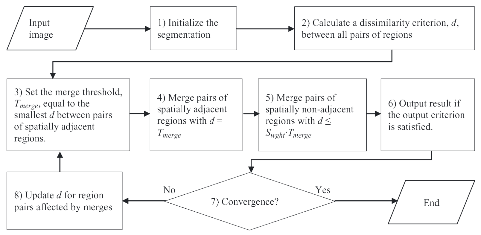
The HSWO approach can be summarized as follows:
- Initialize the segmentation by assigning each image pixel a region label. If a pre-segmentation is provided, label each image pixel according to the pre-segmentation. Otherwise, label each image pixel as a separate region.
- Calculate the dissimilarity criterion value between all pairs of spatially adjacent regions, find the pair of spatially adjacent regions with the smallest dissimilarity criterion value, and merge that pair of regions.
- Stop if no more merges are required. Otherwise, return to step 2.
In the implementation utilized here, all pairs of spatially adjacent regions that have the smallest criterion value are merged in the second step, resolving the issue of “ties.”
The HSWO algorithm produces a globally optimal segmentation result if the statistics at all iterations are independent. However, excellent results are still obtained for natural images, in which the statistics are generally no independent. The sequence of partitions generated from this iterative approach creates a quality hierarchical boundary map of the image, including no scan line dependence. A problem, though, with this HSWO algorithm the large amount of computing time required: more than 30 minutes to process an 256 pixel X 256 pixel image on a 1.2 Ghz computer.
Método de Segmentação Hierárquica com Agrupamento Espectral (HSEG)
Hierarchical Image Segmentation, as presented here, is identical to HSWO with the the addition of a spectral clustering option. Spectral clustering allows the merging of spatially non-adjacent regions, resulting in spatially disjoint regions.
The HSEG algoritmis an image analysis approach that analyzes single band, multispectral, or hyperspectral image data. It can process any image with a resolution up to 8,000 x 8,000 pixels. The implementation of the software analyzes each pixel, groups the pixels that are have similar characteristics to form regions, and then combines regions based on their similarity, whether adjacent or disjointed. This grouping creates spatially disjoint regions. The greater the number of regions located, the higher the segmentation resolution, however some regions may be split into multiple regions when viewing data at its finest levels; the highest resolution is not always ideal.
| 1 | Give each pixel a region label. If a pre-segmentation is provided, label each image according to the pre-segmentation. Otherwise label each pixel as a separate region. | Step 1 initiates the HSEG algorithm by setting the initial region labels for each image pixel. |
| 2 | Calculate the dissimilarity value, dissim_val, between all pairs of spatially adjacent regions. If the spectral clustering weight, spclust_wght > 0.0, also calculate dissim_val for spatially non-adjacent regions. | In step 2, the dissimilarity criterion values for all pairs of spatially adjacent regions are calculated. If spclust_wght > 0.0, the dissimilarity criterion values for all pairs of spatially non-adjacent regions are also calculated. In the implementation, the results with the minimum value of the dissimilarity criterion value for each region are the only results that are saved from the dissimilarity criterion calculations. |
| 3 | Find the smallest dissim_val between all spatially adjacent pairs of regions and set nghbr_thresh equal to it. Set prev_max_threshold = 0.0 and max_threshold = nghbr_thresh. | In step 3, the value of the max_threshold variable is set. This value is output by HSEG to be used in the processing window artifact elmination process. It is also used internally by HSEG to accelerate the region merging process by forcing the region merging threshold to be strictly non-decreasing. The value of prev_max_threshold is also, intialized to 0.0. Along with max_threshold, prev_max_threshold is used in convergence checking step 11. |
| 4 | If spclust_wght = 0.0, go to step 7. Otherwise, if max_threshold = 0.0, merge all pairs of regions with dissim_val=0.0. If max_threshold > 0.0, merge all pairs of regions with dissim_val < spclust_wght*max_threshold. | Step 4 is executed only if spclust_wght > 0.0. If max_threshold > 0.0, only spatially non-adjacent merges will occur. If max_threshold = 0.0, no merges will occur by the dissim_val < spclust_wght*max_threshold test, and spatially adjacent and non-adjacent merges are made by the dissim_val = 0.0 test. |
| 5 | If the number of regions remaining is less than or equal to the preset value chk_nregions, go to step 11. Otherwise, update the dissim_val’s between spatially adjacent pairs of regions as necessary. | Step 5 checks to make sure the number of regions for convergence checking hasn’t already been reached. If not, the dissimilarity criterion values between spatially adjacent region pairs are updated as necessary. |
| 6 | Find the smallest dissim_val between spatially adjacent pairs of regions and set nghbr_thresh equal to it. If nghbr_thresh > max_threshold, set prev_max_threshold = max_threshold and then set max_theshold = nghbr_thresh. | Step 6 finds the smallest dissimilarity criterion value between spatially adjacent regions and sets the threshold variable to it. If the current value of max_threshold is less than nghbr_thresh, the value of prev_max_threshold is updated to the value of max_threshold and value of max_threshold is updated to the value of nghbr_thresh. |
| 7 | Merge all pairs of spatially adjacent regions with dissim_val ≤ max_threshold (update dissim_val’s as necessary). | Step 7 does the merging between spatially adjacent regions and keeps the dissimilarity criterion values updated as necessary. |
| 8 | If the number of regions remaining is less than or equal to the preset value chk_nregions, or if spclust_wght = 0.0, go to step 11. Otherwise, update the dissim_val’s between all pairs of spatially adjacent and non-adjacent regions. | Step 8 checks to make sure the number of regions for convergence checking hasn’t already been reached. If not, if spclust_wght > 0.0, the dissim_val’s between spatially non-adjacent regions are updated as necessary. |
| 9 | Merge all pairs of spatialy adjacent or non-adjacent regions with dissim_val ≤ spclust_wght*max_threshold. (update dissim_val’s as necessary). | Step 9 performs the merging between spatially non-adjacent regions, and keeps the dissimilarity criterion values updated as necessary. |
| 10 | If the number of regions remaining is less than or equal to chk_nregions, go to step 11, else go to step 6. | Step 10 checks to see if convergence checking, step 11, should be executed, and sends the process to step 6 or 11 as appropriate. |
| 11 | If the number of regions remaining is less than or equal to conv_nregions, save the current region label map along with associated region information and STOP. If this is the first this step is executed, save the current region label map with associated region information and go to step 6, else calculate tratio = max_threshold/prev_max_threshold. If tratio is greater than the preset threshold convfact, save the region label map from the previous iteration along with associated region information and go to step 6, else just go to step 6. | Step 11 performs convergence checking. If final convergence has been reached, the appropriate results are output and the algorithm is terminated. Otherwise, convergence checking is performed for determining whether or not the results from the current or previous iteration should be output as a hierarchical level in the segmentation hierarchy output by HSEG. Then the process is returned to step 6. |
Exemplo de HSEG
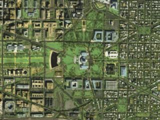 Imagem Original |
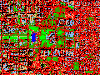 Maior número de regiões |
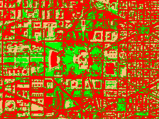 Número Médio de Regiões |
 Menor Número de Regiões |
 Resultado da Segmentação – Número Escolhido de Regiões |
RHSEG
With the addition of alternating iterations of spectral clustering in the HSEG algorithm, the computational demands significantly increase. This is caused primarily because of the requirement to update or calculate the dissimilarity criterion values for all pairs of regions in steps 2 and 8. For a 1024 x 1024 pixel image, this leads to the order of 10000000 comparisons in the initial processing stage.
Nevertheless, this computational obstacle is surmounted by the recursive formulation of the HSEG algorithm, RHSEG. This recursive form not only limits the number of comparisons bwetween spatially non-adjacent regions to a more reasonable number, but also lens itself to a straightforward and efficient implementation on parallel computing platforms.
In regards to the definition of RHSEG, it follows the same as the RHSWO and includes the definition of processing window artifact elimination.
Exemplos de RHSEG
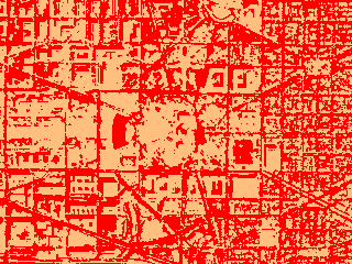
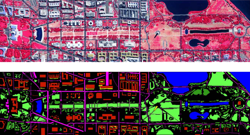
Imagem de Satélite de [1]:
Exemplos da NASA:
![]() (a)
(a)![]()
(b)
![]() (c)
(c)![]()
(d)
Fig. 2. Segmentation results for RHSEG with spclust_wght=0.1, processing window artifact elimination, and with the BSMSE dissimilarity function. (a) Region mean image for the 13 region segmentation result and global dissimilarity value of 9.9326. (b) Hierarchical boundary map for (a). (c) Region mean image for the 9 region segmentation and global dissimilarity value of 11.6204. (d) Hierarchical boundary for (c).